Some tools:

• Stochastic variational inference
• Variance reduction
• Normalizing flows
• Gaussian processes
• Scalable MCMC algorithms
• Semi-implicit variational inference

Bayesian framework

• Bayes theorem:

It defines a rule for uncertainty conversion when new information arrives

• Product rule: any joint distribution can be expressed with conditional distributions

• Sum rule: any marginal distribution can be obtained from the joint distribution by integrating out

• Statistical inference

  Problem: given i.i.d. data \(X=\{x_i\}_{i=1}^n\) from distribution \(p(x\mid\theta)\), estimate \(\theta\)

  1. Frequentist framework: use maximum likelihood estimation (MLE)
  \[\theta_{ML}=\operatorname*{arg\,max}p(X\mid\theta)=\operatorname*{arg\,max}\prod_{i=1}^n p(x_i\mid\theta)=\operatorname*{arg\,max}\sum_i^n\log p(x_i\mid\theta)\]

  Applicability: \(n\ll d\)

  1. Bayesian framework: encode uncertainty about \(\theta\) in a prior \(p(\theta)\) and apply Bayesian inference
  \[p(\theta\mid X)=\frac{\prod_i^n p(x_i\mid\theta)p(\theta)}{\int\prod_i^n p(x_i\mid\theta)p(\theta)d\theta}\]

  Applicability: \(\forall_nd\)

  Advantages: - we can encode prior knowledge/desired properties into a prior distribution - prior is a form of regularization - additionally to the point estimate of \(\theta\), posterior contains information about the uncertainty of the estimate - frequentist case is a limit case of Bayesian one \(\lim_{n/d\to\infty}p(\theta\mid x_1,\dots,x_n)=\delta(\theta-\theta_{ML})\)

Bayesian ML models

In ML, we have \(x\) features (observed variables) and \(y\) class labels or hidden representations (hidden or latent variables) with some model parameters \(\theta\) (e.g. weights of a linear model).

• Discriminative approach, models \(p(y,\theta\mid x)\)

  • Cannot generate new objects since it needs \(x\) as an input and assumes that the prior over \(\theta\) does not depend on \(x\): \(p(y,\theta)=p(y\mid x,\theta)p(\theta)\)
  • Examples: 1) classification/regression (hidden space is small) 2) Machine translation (complex hidden space)

• Generative approach, models \(p(x,y,\theta)=p(x,y\mid\theta)p(\theta)\)

  • It can generate objects (pairs \(p(x,y)\)), but it can be hard to train since the observed space is most often more complicated.
  • Example: Generation of text, speech, images, etc.

• Training

  Given data points \((X_{tr}, Y_{tr})\) and a discriminative model \(p(y,\theta\mid x)\).

  Use the Bayesian framework:

  \[p(\theta\mid X_{tr}, Y_{tr})=\frac{p(Y_{tr}\mid X_{tr},\theta)p(\theta)}{\int p(Y_{tr}\mid X_{tr},\theta)p(\theta) d\theta}\]

  This results in a ensemble of algorithms rather than a single one \(\theta_{ML}\). Ensembles usually performs better than a single model.

  In addition, the posterior captures all dependencies from the training data and can be used later as a new prior.

• Testing

  We have the posterior \(p(\theta\mid X_{tr},Y_{tr})\) and a new data point \(x\). We can use the predictive distribution on its hidden value \(y\)

  \[p(y\mid x, X_{tr},Y_{tr}) = \int p(y\mid x,\theta)p(\theta\mid X_{tr},Y_{tr})d\theta\]

• Full Bayesian inference

During training the evidence \(\int p(Y_{tr}\mid X_{tr},\theta)p(\theta) d\theta\) or in testing the predictive distribution \(\int p(y\mid x,\theta)p(\theta\mid X_{tr},Y_{tr})d\theta\) might be intractable, so it is impractical or impossible to perform full Bayesian inference. In other words, there is not closed form.

Conjugacy

Conjugate distributions

Distribution \(p(y)\) and \(p(x\mid y)\) are conjugate \(\iff\) \(p(y\mid x)\) belongs to the same parametric family as \(p(y)\)

• There’s not conjugacy We can perform MAP to approximate the posterior with \(\theta_{MP}\) since we don’t need to calculate the normalization constant, but we cannot compute the true posterior.

During testing:

Conditional conjugacy

Given the model: \(p(x,\theta)=p(x\mid\theta)p(\theta)\) where \(\theta=[\theta_1,\dots,\theta_m]\)

Conditional conjugacy of likelihood and prior on each \(\theta_j\) conditional on all other \(\{\theta_i\}_{i\neq j}\)

Check conditional conjugacy in practice: For each \(\theta_j\)

• Fix all other \(\{\theta_i\}_{i\neq j}\) (look at them as constants)
• Check whether \(p(x\mid\theta)\) and \(p(\theta)\) are conjugate w.r.t. \(\theta_j\)

Variational Inference

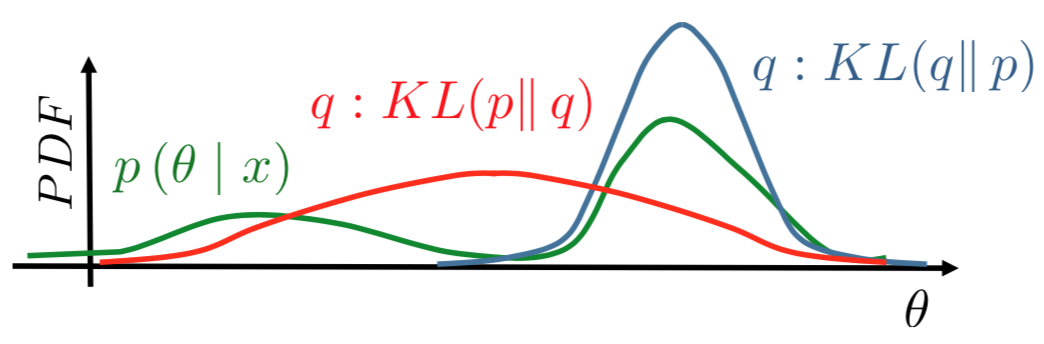
Given the model \(p(x,\theta)=p(x\mid \theta)p(\theta)\), find a posterior approximation \(p(\theta\mid x) \approx q(\theta)\in\mathcal{Q}\), such that:

KL is a good mismatch measure between two distributions over the same domain (see figure). And it has the following properties:

1. \[KL(q\parallel p) \geq 0\]
2. \[KL(q\parallel p)=0 \Leftrightarrow q=p\]
3. \[KL(q\parallel p \neq KL(p\parallel q))\]

Evidence Lower Bound (ELBO) derivation

• Posterior: \(p(\theta\mid x)\)
• Evidence: \(p(x)\), shows the total probability of the observing data.
• Lower bound: \(\log p(x) \geq \mathcal{L}(q(\theta))\)

Note:

• \(\log p(x)\) does not depend on \(q\)
• \(\mathcal{L}\) and \(KL\) depend on \(q\)
• minimizing \(KL\) is the same as maximizing \(\mathcal{L}\).

Optimizing ELBO \(\mathcal{L}\)

Goal: \(\mathcal{L}(q(\theta)) \rightarrow\max_{q(\theta)\in\mathcal{Q}}\)

• Data term: \(\mathbb{E}_{q(\theta)} \log p(x\mid\theta)\)
• Regularizer: \(KL(q(\theta)\parallel p(\theta))\)

Necessary to perform optimization w.r.t. a distribution \(\max_{q(\theta)\in\mathcal{Q}} \mathcal{L}(q(\theta))\). Hard problem! In VI, we approximate with an approximate distribution \(q\). This approximate distribution can belong to a factorized or parametric family.

1. Mean field approximation: Factorized family, \(q(\theta)=\prod_{j=1}^m q_j(\theta_j)\), \(\theta=[\theta_1,\dots,\theta_m]\)
2. Parametric approximation: Parametric family, \(q(\theta)=q(\theta\mid \lambda)\)

Mean Field Approximation

Mean field assumes that \(\theta_1,\dots,\theta_m\) are independent.

• Apply product rule to distribution \(q\): \(q(\theta)=\prod_{j=1}^m q_j(\theta_j\mid\theta_{<j})\)
• Apply i.i.d. assumption: \(q(\theta)=\prod_{j=1}^m q_j(\theta_j)\)

The optimization problem becomes:

This can be solved with block coordinate assent as follows: at each step fix all factors \(\{q_i(\theta_i)\}_{i\neq j}\) except one and optimize w.r.t. to it \(\max_{q_j(\theta_j)}\mathcal{L}(q(\theta))\)

Derivation

So, the optimization problem for step \(j\) is:

Where this happens when:

Block coordinate assent can be described in two steps 1) initialize; 2) iterate

1. Initialize: \(q(\theta)=\prod_{j=1}^m q_j(\theta_j)\)
2. Iterate (repeat until ELBO converge):
   • Update each factor \(q_1,\dots,q_m\): \(q_j(\theta_j)=\frac{1}{Z_j}\exp(\mathbb{E}_{q_{i\neq j}} \log p(x,\theta))\)
   • Compute ELBO \(\mathcal{L}(q(\theta))\)

Note: Mean-field can be applied when we can compute analytically \(\mathbb{E}_{q_{i\neq j}} \log p(x,\theta)\). In other words, applicable when we can compute the conditional conjugacy.

Parametric Approximation

Select a parametric family of variational distributions, \(q(\theta)=q(\theta\mid\lambda)\), where \(\lambda\) is a variational parameter.

The restriction is that we need to select a family of some fixed form, and as a result:

• it might be too simple and insufficient to model the data
• if it is complex enough then there is no guarantee we can train it well to fit the data

The ELBO is:

If we’re able to calculate derivatives of ELBO w.r.t \(\theta\), then we can solve this problem using some numerical optimization solver.

Inference methods

So we have:

1. Full Bayesian inference: \(p(\theta\mid x)\)
2. MAP inference: \(p(\theta\mid x)\approx \delta (\theta-\theta_{MP})\)
3. Mean field variational inference: \(p(\theta\mid x)\approx q(\theta)=\prod_{j=1}^m q_j(\theta_j)\)
4. Parametric variational inference: \(p(\theta\mid x)\approx q(\theta)=q(\theta\mid\lambda)\)

Latent variable model

Mixture of Gaussians

Establish a latent variable \(z_i\) for each data point \(x_i\) that denotes the \(ith\) gaussian where the model was generated.

Model:

where \(\pi_j=p(z_i=j)\) is the prior of the \(jth\) gaussian and \(\theta=\{\mu_j,\sigma^2_j,\pi_j\}_{j=1}^K\) are the parameters to estimate.

Note: If \(X\) and \(Z\) are known, we can use ML. For instance:

• Since \(Z\) is a latent variable, we need to maximize the log of incomplete likelihood w.r.t. \(\theta\).
• Instead of optimizing \(\log p(X\mid \theta)\), we optimize the variational lower bound w.r.t. to both \(\theta\) and \(q(Z)\)
• This can be solved by block-coordinate algorithm a.k.a. EM-algorithm.

Variational Lower Bound: \(g(\xi,\theta)\) is the variational lower bound function for \(f(x)\) iff:

1. For all \(\xi\) for all \(x\): \(f(x)\geq g(\xi,x)\)
2. For any \(x_0\) exists \(\xi(x_0)\) such that: \(f(x_0)=g(\xi(x0),x_0)\)

If we find such variational lower bound, instead of solving \(f(x)\rightarrow\max_x\), we can interatively perform block coordinate updates of \(g(\xi, x)\).

1. \[x_n=\operatorname*{arg\,max}_{x}g(\xi_{n-1},x)\]
2. \[\xi_n=\xi(x_n)=\operatorname*{arg\,max}_{\xi} g(\xi,x_n)\]

Expectation Maximization algorithm We want to solve:

Algorithm: Set an initial point \(\theta_0\)

Repeat iteratively 1 and 2 until convergence

1. E-step, find: \(\begin{align*} q(Z)&=\operatorname*{arg\,max}_{q}\mathcal{L}(q,\theta_0)\\ &=\operatorname*{arg\,max}_{q}{KL}(q\parallel p)\\ &=p(Z\mid X,\theta_0) \end{align*}\)
2. M-step, solve: \(\begin{align*} \theta_*&=\operatorname*{arg\,max}_{\theta}\mathcal{L}(q,\theta)\\ &=\operatorname*{arg\,max}_{\theta}\mathbb{E}_Z \log p(X,Z\mid\theta) \end{align*}\)
   • Set \(\theta_0=\theta_*\) and go to 1

EM monotonically increases the lower bound and converges to a stationary point of \(\log p(X\mid\theta)\), see figure.

Benefits of EM

• In some cases E-step and M-step can be solved in closed-information
• Allow to build more complicated models
• If true posterior \(p(Z\mid X,\theta)\) is intractable, we may search for the closest \(q(Z)\) among tractable distributions by solving optimization problem
• Allows to process missing data by treating them as latent variables
  • It can deal with both discrete and latent variables

Categorical latent variables Since \(z_i\in\{1,\dots,K\}\) the marginal of a mixture of gaussians is a finite mixture of distributions:

• E-step is closed-form: \(q(z_i=k)=p(z_i=k\mid x_i,\theta)=\frac{p(x_i\mid k,\theta)p(z_i=k\mid\theta)}{\sum_{l=1}^Kp(x_i\mid l,\theta)p(z_i=l\mid\theta)}\)
• M-step is a sum of finite terms: \(\mathbb{E}_Z\log p(X,Z\mid\theta)=\sum_{i=1}^n\mathbb{E}_{z_i}\log p(x_i,z_i\mid\theta)=\sum_{i=1}^n\sum_{k=1}^K q(z_i=k)\log p(x_i,k\mid\theta)\)

Continuous latent variables A mixture of continuous distributions

• E-step: only done in closed form when conjugate distributions, otherwise the true posterior is intractable

  \[q(z_i)=p(z_i\mid x_i,\theta)=\frac{p(x_i\mid z_i,\theta)p(z_i\mid\theta)}{\int p(x_i\mid z_i,\theta)p(z_i\mid\theta) dz_i}\]

Typically continuous latent variable are used for dimensionality reduction a.k.a. representation learning

Log-derivative trick

For example, we commonly find expressions as follows:

Now, the first term can be replaced with Monte Carlo estimate of expectation. Using the log-derivative trick, the second expectation can also be estimated via Monte Carlo.

Score function

It is the gradient of the log-likelihood function with respect to the parameter vector. Since it has zero mean, the value \(z_i^*\) in \(\nabla_{\phi}\log q(z_i^*\mid\theta)\) oscillates around zero.

Proof it has zero mean:

REINFORCE