Expectation Propagation Notes

Commonly in probabilistic models, we deal with expectations that are either too hard to compute or intractable. In Bayesian inference setting, we usually need to calculate the posterior \(p(z\mid x)\) for parameter estimation or the evidence \(p(x)\) for model selection, where \(z\) is a latent variable and \(x\) is known. We can use approximate inference to solve this complex integrals. There is many work that have been done in this area, but approximate methods can be classified in deterministic and sampling methods. The former evaluates the integral in several locations and constructs an approximate function. The latter relies in the law of large numbers and given enough samples, the integral will converge to the true value.

1. Sampling methods: Monte Carlo methods such as Importance sampling, Gibbs sampling, MCMC
2. Deterministic methods: Variational inference, Laplace approximation, Expectation Propagation

This notes include explanations for ADF and Expectation Propagation.

Assumed-density Filtering (ADF)

ADF (aka. moment matching, online Bayesian learning and weak marginalization) can be used when given the joint \(p(x, z)\), we want to calculate the posterior over the latent variable \(p(z \mid x)\) and the evidence \(p(x)\). This is a common task in statistical machine learning where we want to fit a parametric distribution.

The common setting: we are given a set of data points \(D=x_1,\dots,x_n\), which we assume are i.i.d. Thus, we can model the joint distribution as the product of its observations and the prior \(p(D,z) = p(z)\prod_i p(x_i\mid z)\).

1. Factorization: We can factorize the joint distribution as needed, but it is recommendable that each factor is simple enough for being propagated. Also the fewer terms, entails fewer approximations. In general, we can define the joint distribution as follows where \(t_0\) is the prior.

   \[p(D,z) = \prod_{i=0}^n t_i(z)\]

2. Choose a parametric approximating distribution: our goal is to approximate the posterior with a simple distribution; \(p(z\mid D) \approx q(z)\).

   • This distribution has to belong to the exponential family, so we can propagate its sufficient statistics.
   • Pick \(q\) based in the nature and domain of \(z\).

3. Incorporate each \(t_i\) term: Sequence and incorporate the term \(t_i\) into the approximate posterior \(q(z\)) going from an old posterior to a new posterior.

   • incorporate: \(\hat p(z) = \frac{q(z)t_i(z)}{\int_z q(z)t_i(z) dz}\)
   • from old to new: \(\min D_{KL}(\hat p \parallel q^{new})\), which equivalent to match the moments.

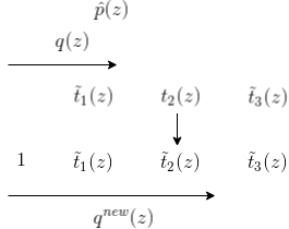
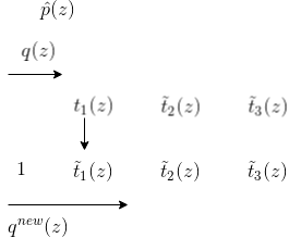
Intuition

Here is a graphical example of ADF in practice.

1. \(q(z)\) can be initialized to \(1\), and it’s not necessary to approximate.

1. Incorporate \(t_1\), resulting in a one-step step posterior \(\hat p\). We approximate \(\hat p\) with \(q^{new}\).

1. Repeat step 2, including \(t_2\).

We can notice that there’s a dependence in the order of the data points; order matters.

The error of ADF tend to increase when similar data points are processed

Expectation Propagation

Expectation Propagation (Minka., NIPS 2001) is a generalization of ADF. We can notice that ADF is an iterative method that performs a one-pass to all data points. EP solves this problem by performing iterative refinements.

ADF:

1. Treat \(t_i\) as it is.
2. Approximate \(q(z)\).

EP:

1. Approximate \(t_i\) with \(\tilde t_i\).
2. Use exact posterior

This refinements are always possible. It is the ratio of the new posterior to the old posterior times a constant:

Let’s see how this looks in practice:

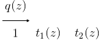
First, let’s derive an intuition of ADF using \(\tilde t_i\).

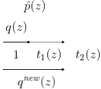
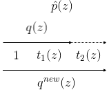
1. We approximate \(t_1\) with \(\tilde t_1\) using the prior \(t_0=1\)m and go from \(q^{old}\) to \(q^{new}\).

2.